Quickstart
CLI
From version 1.0.10 there’s a suggested analysis pipeline in the form of a CLI tool to facilitate usage. To use it, create a script like the following, and run it:
from scludam import launch

if __name__ == "__main__":
    launch()
From there, you can download data from GAIA, load a file, run the analysis pipeline, plot and save results.
NOTES:
For plotting to display correctly, you need to have the corresponding library installed, such as PyQt6 in your environment.
The CLI tool is still rudimentary, it will exit on some incorrect inputs. Follow the directions of the prompts carefully.
Main functionality example
1import matplotlib.pyplot as plt
2
3from scludam import DEP, CountPeakDetector, HopkinsTest, Query, RipleysKTest
4
5# search some data from GAIA
6# with error and correlation
7# columns for better KDE
8df = (
9 Query()
10 .select(
11 "ra",
12 "dec",
13 "ra_error",
14 "dec_error",
15 "ra_dec_corr",
16 "pmra",
17 "pmra_error",
18 "ra_pmra_corr",
19 "dec_pmra_corr",
20 "pmdec",
21 "pmdec_error",
22 "ra_pmdec_corr",
23 "dec_pmdec_corr",
24 "pmra_pmdec_corr",
25 "parallax",
26 "parallax_error",
27 "parallax_pmra_corr",
28 "parallax_pmdec_corr",
29 "ra_parallax_corr",
30 "dec_parallax_corr",
31 "phot_g_mean_mag",
32 )
33 # search for this identifier in simbad
34 # and bring data in a circle of radius
35 # 1/2 degree
36 .where_in_circle("ngc2168", 0.5)
37 .where(("parallax", ">", 0))
38 .where(("phot_g_mean_mag", "<", 18))
39 # include some common criteria
40 # for data precision
41 .where_arenou_criterion()
42 .where_aen_criterion()
43 .get()
44 .to_pandas()
45)
46
47# If data already has been downloaded, you can load it from a file:
48# > from astropy.table.table import Table
49# > df = Table.read("path_to_my_file/ngc2168_data.fits").to_pandas()
50
51
52# Build Detection-Estimation Pipeline
53dep = DEP(
54 # Detector configuration for the detection step
55 detector=CountPeakDetector(
56 bin_shape=[0.3, 0.3, 0.07],
57 min_score=3,
58 min_count=5,
59 ),
60 det_cols=["pmra", "pmdec", "parallax"],
61 sample_sigma_factor=2,
62 # Clusterability test configuration
63 tests=[
64 RipleysKTest(pvalue_threshold=0.05, max_samples=100),
65 HopkinsTest(),
66 ],
67 test_cols=[["ra", "dec"]] * 2,
68 # Membership columns to use
69 mem_cols=["pmra", "pmdec", "parallax", "ra", "dec"],
70).fit(df)
71
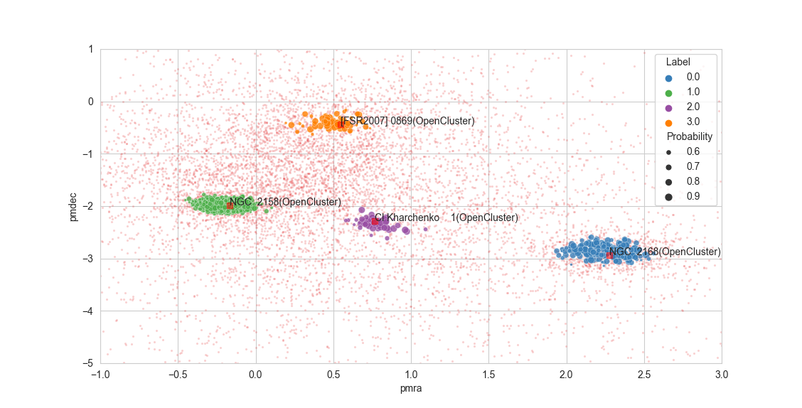
72# plot the results
73dep.scatterplot(["pmra", "pmdec"])
74# zoom on interesting area
75plt.axis([-1, 3, -5, 1])
76plt.show()
77
78# write results to file
79dep.write("ngc2168_result.fits")
Documentation quick guide
Building queries for GAIA catalogues and retrieving data:
QueryDetection and membership estimation pipeline:
DEPDetection method:
CountPeakDetectorClusterability tests:
stat_testsClustering method:
SHDBSCANProbability Estimation:
DBMEKernel Density Estimation with per-observation or per-dimension bandwidth, plugin or rule-of-thumb methods:
HKDE
Documentation module guide
Query building, SIMBAD object searching and data related functionality:
fetcherDetection and membership estimation pipeline:
pipelineDetection:
CountPeakDetectorClusterability tests:
stat_testsClustering:
shdbscanProbability estimation:
membershipKernel Density Estimation:
hkdeUtils such as GAIA column names interpretation and one hot encoding:
utilsCustom ploting functions:
plotsUtils for R communication:
rutilsUtils for masking data:
maskerUseful distributions for data generation:
synthetic