scludam.stat_tests module

Module for useful statistical tests.

The tests in this module can be used to determine if there is cluster structure (the data is “clusterable”) in a n dimensional numerical dataset.

class scludam.stat_tests.TestResult(rejectH0: bool)

Bases: object

Base class to hold the results of a statistical test.

Variables:

rejectH0 (bool) – Whether the null hypothesis was rejected.

class scludam.stat_tests.StatTest

Bases: object

Base class for statistical tests.

abstract test(data: ndarray[Any, dtype[number]][ndarray[Any, dtype[number]]], *args, **kwargs) → TestResult

Perform the test.

Parameters:

data (Numeric2DArray) – numpy numeric 2d array with the data to be tested.

Returns:

Test result. Its fields depend on the specific test.

Return type:

TestResult

class scludam.stat_tests.HopkinsTestResult(rejectH0: bool, value: Number, pvalue: Number)

Bases: TestResult

Results of a Hopkins test.

Variables:

• rejectH0 (bool) – True if the null hypothesis is rejected.

• pvalue (Number) – The p-value of the test.

• value (Number) – The value of the Hopkins statistic.

class scludam.stat_tests.HopkinsTest(sample_ratio: int = 0.1, max_samples: int = 100, metric: str | DistanceMetric = 'euclidean', n_iters: int = 100, threshold: Number | None = None, pvalue_threshold: float = 0.05)

Bases: StatTest

Class to perform a Hopkins spatial randomness test.

Variables:

• n_iters (int, optional) – Number of iterations to perform the test. Final Hopkins statistic result is taken as the median of the results, by default is 100.

• sample_ratio (float, optional) – Sample ratio to take from the data, by default is 0.1. The number of samples is n*sample_ratio.

• max_samples (int, optional) – Number of max samples to take from the data, by default is 100. If n_samples is greater than this value, it is set to this value.

• metric (Union[str, DistanceMetric], optional) – Metric to use for the distance between points, by default is ‘euclidean’. Can be str or sklearn.neighbors.DistanceMetric.

• threshold (Number, optional) – Threshold to use with the Hopkins statistic value to define if H0 is rejected, by default is None. If set, it is used instead of the pvalue_threshold.

• pvalue_threshold (float, optional) – Threshold to use with the p-value to define if H0 is rejected, by default is 0.05.

Notes

The test compares the distance between a sample of m points X' from the data set X and their nearest neighbors in X, to the distances from X to their nearest neighbors in a uniform distribution. The null hypothesis is:

• H0: The dataset X comes from a Poisson Point Process.

Which can be thought of as:

• H0: The dataset X does not present cluster structure.

The formula to calculate the Hopkins statistic [1] is h = sum(d1**l) / (sum(d1**l) + sum(d2**l)), where:

• d1: distance_to_nearest_neighbor_in_X

• d2: distance_to_nearest_neighbor_in_uniform_distribution

• l: dimensionality of the data

The Hopkins statistic is a number between 0.5 and 1. A value ~0.5 supports the null hypothesis. A value ~1.0 supports the alternative hypothesis. To get the p-value, the statistic is compared to a beta distribution with parameters (m, m).

References

[1]

Hopkins, B. and Skellam, J.G. (1954). A new method of determining the type of distribution of plant individuals”. Annals of Botany, 1954, 18(2), pp.213-227. https://doi.org/10.1093/oxfordjournals.aob.a083391

Examples

from sklearn.datasets import load_iris

from scludam import HopkinsTest

iris = load_iris().data

ht = HopkinsTest().test(data=iris)
print(ht)
#  >> HopkinsTestResult(rejectH0=True, value=0.9741561806256851, pvalue=2.220446049250313e-16)

test(data: ndarray[Any, dtype[number]][ndarray[Any, dtype[number]]], *args, **kwargs)

Perform the Hopkins test.

Parameters:

data (Numeric2DArray) – Array containing the data.

Returns:

Test results.

Return type:

HopkinsTestResult

class scludam.stat_tests.DipDistTestResult(rejectH0: bool, value: Number, pvalue: Number, dist: ndarray[Any, dtype[number]][ndarray[Any, dtype[number]]])

Bases: TestResult

Results of a dip dist test.

Variables:

• value (Number) – The value of the dip statistic.

• pvalue (Number) – The pvalue of the test.

• dist (Numeric1DArray) – The ordered distance array.

class scludam.stat_tests.DipDistTest(max_samples: int = 1000, metric: str = 'euclidean', pvalue_threshold: float = 0.05)

Bases: StatTest

Class to perform a Dip-Dist test of multimodality over pairwise distances.

The Dip-Dist implementation is based on the Python Dip test wrapper built by Ralph Ulrus, [2].

Variables:

• max_samples (int, optional) – Maximum number of samples to use, by default is 1000. If there are more data points than max_samples, then the data is sampled.

• metric (Union[str, DistanceMetric], optional) – Metric to use for the distance between points, by default is ‘euclidean’. Can be str or sklearn.neighbors.DistanceMetric.

• pvalue_threshold (float, optional) – Threshold to use with the p-value to define if H0 is rejected, by default is 0.05.

Notes

The test analyzes the pairwise distance distribution [3] between points in a data set to determine if said distribution is multimodal. The null hypothesis is:

• H0: The distance distribution is unimodal.

Which can be thought of as:

• H0: The data set X does not present cluster structure.

More specifically, the distance distribution will be unimodal for uniform data distributions or single cluster distributions. It will be multimodal when there are several clusters or when there is an aggregate of a uniform distribution and a cluster. The Hartigan’s Dip statistic [4] can be defined as the maximum difference between an empirical distribution and its closest unimodal distribution calculated using the greatest convex minorant and the least concave majorant of the bounded distribution function.

References

[3]

R. Urlus (2022). A Python/C(++) implementation of Hartigan & Hartigan’s dip test for unimodality. https://pypi.org/project/diptest/

[2]

A. Adolfsson, M. Ackerman, N. C. Brownstein (2018). To Cluster, or Not to Cluster: An Analysis of Clusterability Methods . https://doi.org/10.48550/arXiv.1808.08317

[4]

J. A. Hartigan and P. M. Hartigan (1985). The Dip Test of Unimodality. Annals of Statistics 13, 70–84. D OI: 10.1214/aos/1176346577

Examples

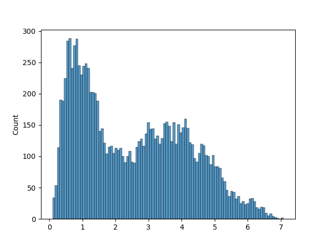
import matplotlib.pyplot as plt
import seaborn as sns
from sklearn.datasets import load_iris

from scludam import DipDistTest

iris = load_iris().data

dd = DipDistTest().test(data=iris)
print(dd)
#  >> DipDistTestResult(rejectH0=True, value=0.01415416887708115, pvalue=0.0, dist=array([0.1, ..., 7.08519583]))
sns.histplot(dd.dist, bins=100)
plt.show()

test(data: ndarray[Any, dtype[number]][ndarray[Any, dtype[number]]], *args, **kwargs)

Perform the Dip-Dist test.

Parameters:

data (Numeric2DArray) – numpy 2d numeric array containing the data.

Returns:

The test results.

Return type:

DipDistTestResult

class scludam.stat_tests.RipleyKTestResult(rejectH0: bool, value: Number, radii: ndarray[Any, dtype[number]][ndarray[Any, dtype[number]]], l_function: ndarray[Any, dtype[number]][ndarray[Any, dtype[number]]])

Bases: TestResult

Results of a Ripley’s K test.

Variables:

• rejectH0 (bool) – True if the null hypothesis is rejected.

• value (Number) – The value calculated to determine if H0 is rejected. If the test mode is chiu or ripley, then the value is the the supremum statistic. If the test mode is ks, then the value is the pvalue of the Kolmogorov-Smirnov test.

• radii (Numeric1DArray) – The radii used in the test.

• l_function (Numeric1DArray) – The L function values.

class scludam.stat_tests.RipleysKTest(rk_estimator: RipleysKEstimator | None = None, used_fitted_rk_estimator: RipleysKEstimator | None = None, scaler: TransformerMixin = MinMaxScaler(), mode: str = 'ripley', radii: ndarray[Any, dtype[number]][ndarray[Any, dtype[number]]] | None = None, factor: float | None = None, pvalue_threshold: float = 0.05, max_samples: int = 5000)

Bases: StatTest

Class to perform the Ripleys K test of 2D spatial randomness.

Variables:

• rk_estimator (astropy.stats.RipleysKEstimator, optional) – Estimator to use for the Ripleys K function [5], by default is None. Only used if a custom RipleysKEstimator configuration is needed.

• mode (str, optional) –

  The comparison method to use to determine the rejection of H0, by default is “ripley”. Allowed values are:

  1. ”ripley”: H0 rejected if s > ripley_factor * sqrt(area) / n where

     • area: is the area of the 2D data set taken as a square window.

     • n: is the number of points in the data set.

     • ripley_factor: are the tabulated values calculated by Ripleys [5] to determine p-value significance. Available Ripleys factors are p-value = 0.05 -> factor = 1.42 and p-value = 0.01 -> factor = 1.68.

  2. ”chiu”: H0 rejected if s > chiu_factor * sqrt(area) / n where:

     • chiu_factor: are the tabulated values suggested by Chiu [6] to determine p-value significance. Available Chiu factors are p-value = 0.1 -> factor = 1.31, p-value = 0.05 -> factor = 1.45 and p-value = 0.01 -> factor = 1.75.

  3. ”ks”: H0 rejected if kolmogorov_smirnov_test_pvalue < pvalue_threshold, where kolmogorov_smirnov_test_pvalue is the p-value of the Kolmogorov Smirnov test comparing the estimated L function to the theoretical L function of a uniform distribution. This option is experimental and should be used with caution.

• radii (Numeric1DArray, optional) –

  numpy 1d numeric array containing the radii to use for the Ripleys K function, by default is None. If radii is None, radii are taken in a range [0, max_radius], where max_radius is calculated as:

  • recommended_radius = short_side_of_rectangular_window / 4

  • recommended_radius_for_large_data_sets = sqrt(1000 / (pi * n))

  • max_radius = min(recommended_radius, recommended_radius_for_large_data_sets)

  The steps between the radii values are calculated as step = max_radius / 128 / 4. This procedure is the recommended one in R spatstat package [7].

• max_samples (int, optional) – The maximum number of samples to use for the test, by default is 5000. If the dataset has more than max_samples, then the test is performed on a random sample of max_samples.

• factor (float, optional) – The factor to use to determine the rejection of H0, by default is None. If factor is provided, then pvalue_threshold is ignored.

Raises:

ValueError – If tabulated factor for the chosen p-value threshold is not available, or if the chosen p-value threshold is invalid.

Notes

The test calculates the value of an estimate for the L function [8] (a form of Ripleys K function) for a set of radii taken from the center of the data set, and compares it to the theoretical L function of a uniform distribution. The null hypothesis is:

• H0: The data set X comes from a Poisson Point Process.

Which can be thought of as:

• H0: The data set X does not present cluster structure.

The Ripleys K(r) function is defined as the expected number of additional random points within a distance r of a typical random point. For a completely random point process (Poisson Point Process), K(r) = pi*r^2. The L(r) function is a form of K(r) defined as L(r) = sqrt(K(r)/pi). The statistic to define if H0 is rejected based on the L function is the supremum of the difference s = max(L(r) - r).

References

[5] (1,2)

B. D. Ripley (1979). Tests of Randomness for Spatial Point Patterns. J. R. Statist. Soc. B (1979), 41, No.3, pp. 368-374. https://doi.org/10.1111/j.2517-6161.1979.tb01091.x

[6]

S. N. Chiu (2007). Correction to Koen’s critical values in testing spatial randomness. Journal of Statistical Computation and Simulation 2007 77(11-12):1001-1004. DOI: 10.1080/10629360600989147

[7]

A. Baddeley, R. Turner (2005). Spatstat: An R Package for Analyzing Spatial Point Patterns. Journal of Statistical Software, 12(6), 1–42. DOI: 10.18637/jss.v012.i06.

[8]

J. Besag (1977). Contribution to the Discussion on Dr. Ripley’s Paper. Journals of the Royal Statistical Society, B39, 193-195.

Examples

import matplotlib.pyplot as plt
import seaborn as sns
from sklearn.datasets import load_iris

from scludam import RipleysKTest

iris = load_iris().data

rk = RipleysKTest().test(data=iris[:, 0:2])
print(rk)
#  >> RipleyKTestResult(rejectH0=True, value=0.07193140227503197, radii=array([0., ..., 0.25]), l_function=array([0., ..., 0.31045381]))
sns.lineplot(
    x=rk.radii,
    y=rk.l_function,
    linestyle="--",
    color="red",
    label="Estimated L function",
)
sns.lineplot(
    x=rk.radii,
    y=rk.radii,
    color="k",
    label="Theoretical Poisson Point Process L function",
)
plt.show()

test(data: ndarray[Any, dtype[number]][ndarray[Any, dtype[number]]], *args, **kwargs)

Perform the Ripleys K test of 2D spatial randomness.

Parameters:

data (Numeric2DArray) – numpy 2d numeric array containing the data set to test.

Returns:

Result of the Ripleys K test.

Return type:

RipleysKTestResult

Warns:

UserWarning – Warns if some dataset points are repeated (exactly equal). In that case, the RipleysKEstimator will not be able to calculate the L function, so repeated points will will be eliminated before the test. Bound to change when RipleysKEstimator implementation is changed.